How Guinness led to improvements in statistics which, in turn, led to improved Guinness.

As you linger over a Black and Tan at your favorite pub, take a moment to contemplate the significance of significance. How do you decide what’s true and what’s coincidence? Will that diet pill really help you lose weight? Is Brand Y really better than Brand X in some specified way? If plastic is substituted for metal in a car body, will it be just as safe in a crash and will it give better mileage? If the issue is diet pills or brand comparison, you might be satisfied with celebrity endorsements.

But for the things that really matter, like medical treatments, or products which fall under the jurisdiction of regulatory agencies like product safety, some type of formal testing is needed to prove the claim.

In an ideal world, product testing would be simple because measurements under the same conditions would give the same results every time. In the real world, lots of unknown factors cause the results to vary in even well-controlled tests. We need a way to decide when the differences are large enough to be considered real as opposed to just “the luck of the draw.” We also need some way of quantifying how confident we are in our conclusions. To achieve strong conclusions in testing, we must apply the theory of statistics.

Who didn’t love their first statistics course?

Anyone who has suffered through an introductory statistics course has seen (and hopefully remembered) the following version of statistical testing.

Hypothesis Testing using the example of statistically evaluating car mileage

1. Make a hypothesis (called the null hypothesis) about how the test will come out: Car Model A has the same average mileage as Model B.
2. Make an alternate hypothesis: Model A has better mileage than Model B.
3. Test the samples: Take a sample of cars of each model and run them over the same course.
4. This part is easy. Compare the results: The difference in mean mileage between the samples is compared with the random distribution for the sample difference, calculated under the null hypothesis (no difference) based on the variability within each sample. If the probability of seeing a difference as large as or larger than the one observed is small enough, we reject the null hypothesis and accept the alternate.*

*Students often find this construction a bit awkward, since you reject the null hypothesis to accept the result you want to test for.

This approach to statistical hypothesis testing was first described by Ronald Fisher in a 1925 paper. However, we still need to decide what probability of seeing a difference is “small enough.” Formally, it is the probability of incorrectly rejecting the null hypothesis and is termed statistical significance. In statistical notation, it is designated by the Greek letter alpha (α). Its importance is that it gives a quantitative estimate of how uncertain (or conversely, how certain) we are in our decision.

Fisher suggested using a probability value of 0.05 (one chance of error in 20) for alpha, and it is still the go-to value in most scientific publications (which means that one in 20 conclusions are probably wrong). These are, perhaps, decent odds in a single test for academic exploratory research, but in other cases (e.g. medical treatments) the consequences of making an error are great enough to require more confidence in the results. In cases like that, alpha may be set to 0.01 or 0.001. There are also many situations where a lot of tests or comparisons are needed. In those cases, the probability of making this kind of error (called type I) goes up dramatically. When the number of comparisons is very large, the significance has to be set very low. In particle physics it is typically about 0.00000003, while in genome-wide association studies 0.000000005 is the standard.

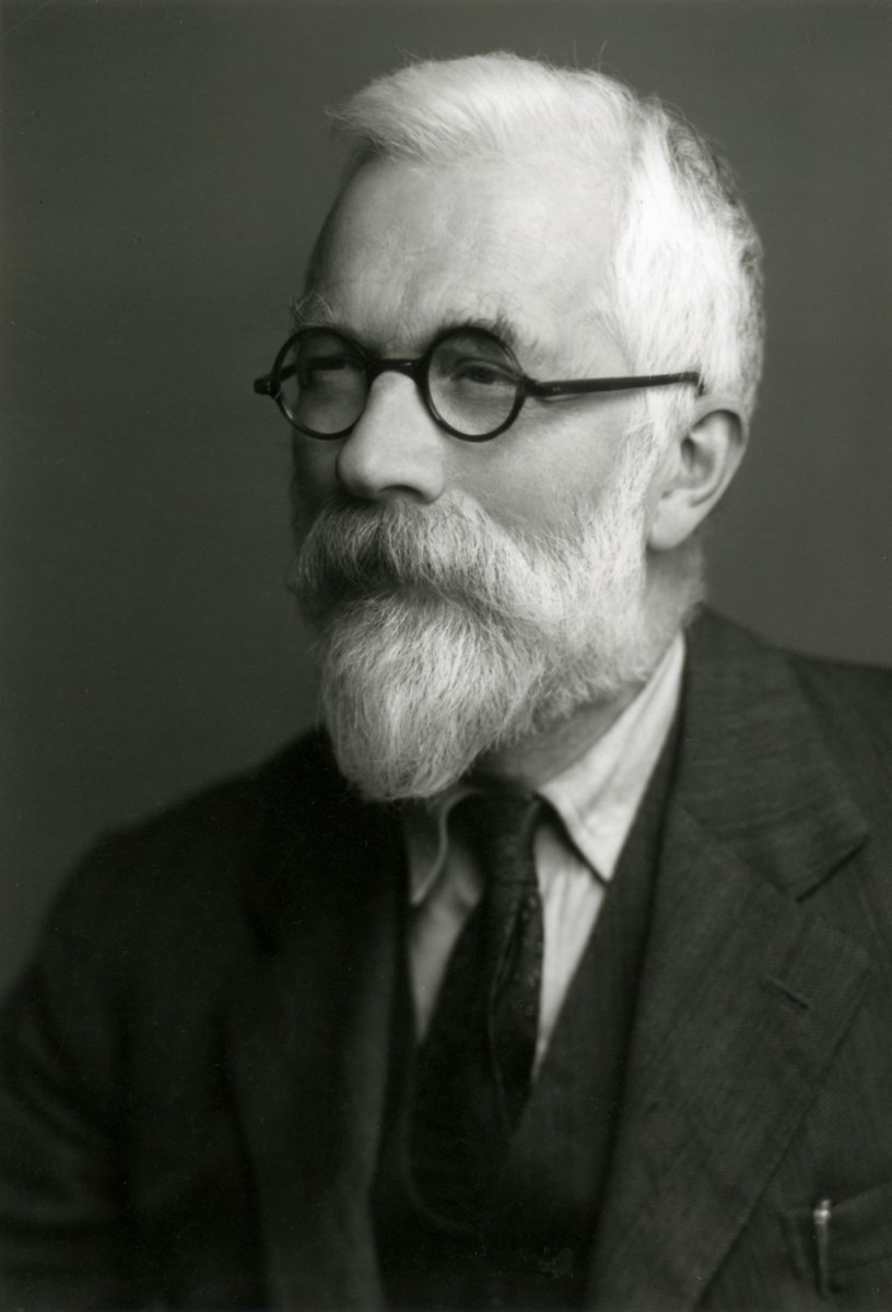
Ronald Fisher, father of ye olde p-value

Note that this method also relies on being able to calculate the probability of distribution of the test statistic. When the statistic is the difference in sample means, as in the case above, we catch a lucky break because of what’s called the central limit theorem. Put simply, the theorem says for large sample sizes the difference in sample means will follow a normal distribution (does bell curve ring a bell?) regardless of the distribution of values within the samples. Note if the sample size is large enough. Sampling can be expensive.

This is where Guinness enters the story (you’ve been waiting).

Guinness became an Irish brewery specializing in Porter style beer

Arthur Guinness started brewing ales in Dublin in 1759. He had started a brewery ten miles outside of town four years earlier with an inheritance from his godfather, an Archbishop of Cashel, but moved to take a 9,000 year lease (clearly an optimist!) on an existing brewery on 4 acres in the city. It wasn’t until 1778 that he first sold a strong dark style of beer, called porter, which had become popular in London. This was the first type of London beer to be aged at the brewery and fit to drink on delivery. By the end of the century, Arthur had expanded his brewery and switched to brewing only porter. The strongest porters came to be called stouts and, from the 1840’s through much of its history, the Guinness brewery produced only three variations of that single beer type: porter, single stout and double stout.

Throughout the 19th and early 20th centuries, the Guinness & Son brewery expanded with increasing rapidity. In 1838 it was the largest brewery in Ireland and, in 1886, the largest in the world. On the eve of WWI, it supplied 10% of the beer sold in the UK. By the 1930’s it had become the seventh largest company in the world.

With that kind of scale-up, improving production methods while maintaining batch-to-batch consistency and developing sources for ingredients becomes an on-going struggle requiring more than the traditional brewmaster’s art. The London porter producers had already pioneered the use of scientific instruments like the thermometer (~1760) and hydrometer (1770) in brewing.

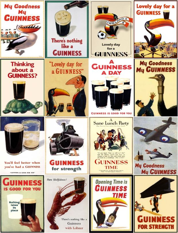
Guinness: The Statistician’s Beer

In 1893, Guinness hired its first university science graduate, and in 1901 it established a research laboratory, followed quickly by an experimental brew house and experimental maltings. In 1899, William S. Gosset, a graduate of college studies in mathematics and chemistry, joined the company to help control beer quality and determine the highest yielding barley varieties. Gosset turned to statistics for guidance, but beer batches and barley fields are expensive investments, so he had to make do with much smaller samples than those of the biometrical statisticians of that era. In 1906-1907, Gossett enlisted the help of one such statistician, Karl Pearson, in developing the mathematics of small-sample methods.

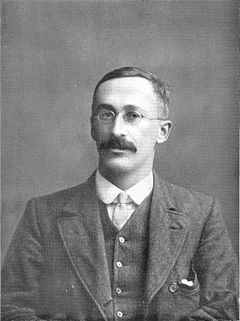
William Gosset: The man behind Student’s t-test

Gosset believed his results would be broadly useful but, because a former employee had published company trade secrets, Guinness had a policy against employee publication. He was eventually able to gain an exception although, in order to avoid creating envy among fellow employees, he published under the pseudonym Student. Thus, we have the Student’s t-test, familiar to all statistics students (no pun intended), while Gosset’s name is known to few. Pearson did not recognize the importance of Gosset’s work, but Fisher (remember him?) did. It fit in well with Fisher’s construct, degrees of freedom, another foundational concept in statistics.

The work of Fisher and Gosset provided important tools for the application of statistical testing to practical problems (and important work for the quality of that beloved beer).

Ultimately other approaches to hypothesis testing proved more useful for advancing statistical theory. Use of a 0.05 significance level as a gatekeeper for publishable research has proven problematic. It is thought to be one of the reasons a large percentage of published biomedical and social sciences results are not reproducible.

In March 2016, the American Statistical Association issued a statement cautioning against the misuse and misinterpretation of statistical significance and p-values. The statement points out that good scientific and engineering practice requires proper study design and conduct, as well as a variety of numerical and graphical summaries of the results. Most especially, it states there is no substitute for “understanding of the phenomenon under study, interpretation of results in context, complete reporting and proper logical and quantitative understanding of what data summaries mean.” In other words, there is no simple tool which can substitute for knowledge and experience.

Beer and statistics: Improving each other since c. 1906

These difficulties aside, the pioneering work of Fisher and Gosset helped usher in the era of statistical testing so essential to modern engineering and production. It seems appropriate to raise your glass to their truly significant achievements.